ColorMAE: Exploring data-independent masking strategies in Masked AutoEncoders
We design data-independent masking for MAE by filtering Noise.
King Abdullah University of Science and Technology (KAUST), GenAI Center of Excellence
We design data-independent masking for MAE by filtering Noise.
King Abdullah University of Science and Technology (KAUST), GenAI Center of Excellence

Current Data-dependent Masking approaches for MAE allow for the extraction of better feature representations but come with additional computational costs. In contrast, data-independent masking approaches do not incur additional computational costs, although they result in lower visual representations. Can we enhance MAE performance beyond random masking without relying on input data or incurring additional computational costs?
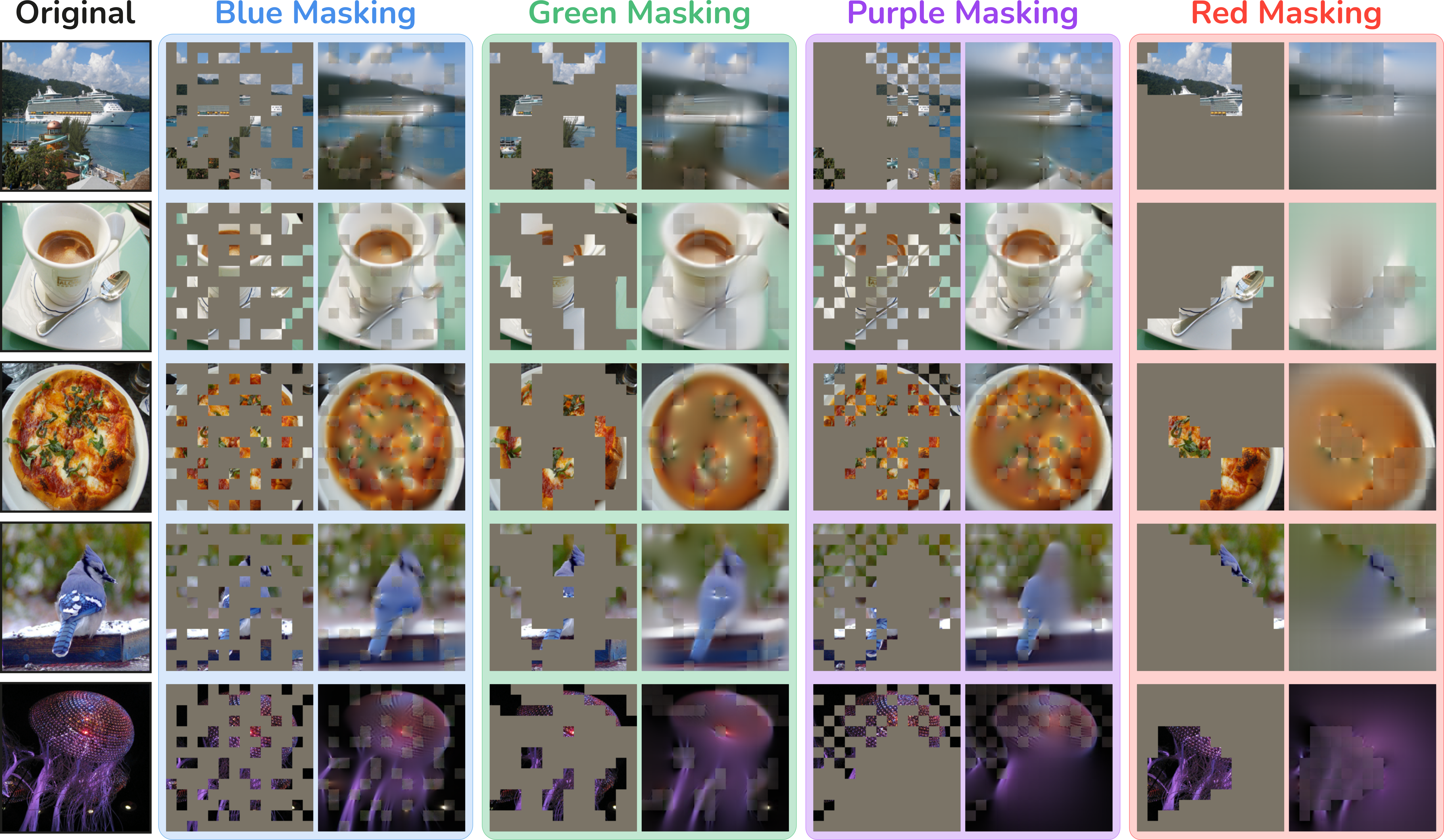
We introduce ColorMAE, a simple yet effective data-independent method which generates different binary mask patterns by filtering random noise. Drawing inspiration from color noise in image processing, we explore four types of filters to yield mask patterns with different spatial and semantic priors. ColorMAE requires no additional learnable parameters or computational overhead in the network, yet it significantly enhances the learned representations.

In image processing, the concept of color noise refers to different types of noise, each characterized by a unique frequency distribution, such as predominance in the low-frequency band. Inspired by this concept, we introduce a simple yet effective data-independent method, termed ColorMAE, which generates binary mask patterns by filtering random noise. We explore four types of filters to yield mask patterns with different spatial and semantic priors. To align with traditional terminology in image processing, we categorize the produced random patterns as Red, Blue, Green, and Purple noise.
Let $W(x, y)$ represent a random noise image, where $x$ and $y$ are spatial coordinates. We apply a blurring operation over $W$ using a Gaussian kernel $G_{\sigma}$ with standard deviation $\sigma$ to filter out the high-frequency components and accentuate low frequencies effectively. This operation transforms the random noise into red noise $N_r$ given by:
$$ N_r = G_\sigma * W, $$
where $*$ denotes the convolution operation.
To generate blue noise patterns, it is required to apply a high-pass filter over $W$. A practical approach to implementing a high-pass filter involves first applying a low-pass filter $(G_\sigma * W)$ to obtain the low-frequency content. Then, this filtered output is subtracted from the original random noise image $W$, effectively retaining the high-frequency components. The resulting blue noise $N_b$ is formally expressed as
$$ N_b = W - G_\sigma * W. $$
This noise is defined as the mid-frequency component of white noise; i.e., it can be generated by applying a band-pass filter over $W$ to eliminate both high and low frequencies. Such band-pass filtering effect can be approximated by sequentially applying two Gaussian blurs: first, a weak blur is applied to $W$ to remove the highest frequency details, followed by a separate strong blur to capture the lowest frequency content of $W$. By subtracting the strongly blurred version of $W$ from the weakly blurred one, the resultant noise image retains only the mid-frequency components. Formally, the green noise $N_g$ image can be obtained as
$$ N_g = G_{\sigma_1} * W - G_{\sigma_2} * W, $$
where $\sigma_1$ and $\sigma_2$ denote the standard deviation of the two Gaussian kernels with $\sigma_1 < \sigma_2$.
Finally, in this work, we refer to purple noise as the noise that has only high and low-frequency content, i.e., does not have a middle-frequency component. We apply a band-stop filter over the random noise $W$ to produce this type of noise. Specifically, we first apply a band-pass filter to $W$ to obtain green noise and then subtract it from the input $W$, preserving only the low and high frequencies. Formally, this transformation of the noise $W$ into purple noise $N_p$ can be expressed as
$$ N_p = W - (G_{\sigma_1} * W - G_{\sigma_2} * W), $$where $\sigma_1 < \sigma_2$. Analyzing the periodogram (P) in the above Figure (column "Purple"), we can observe that this noise combines the characteristics of both red and blue noise.
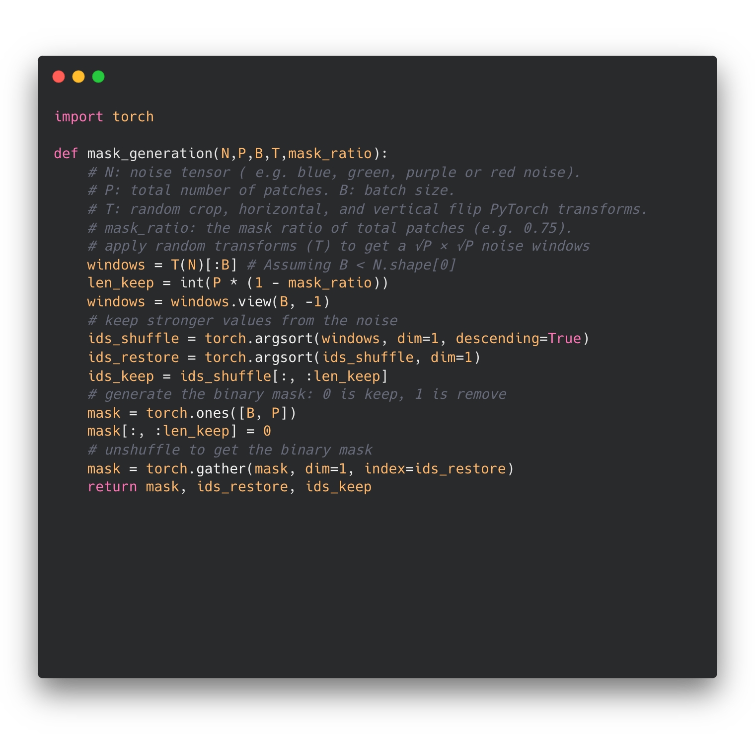
In implementation, we pre-compute color noise offline and store them in GPU memory before initiating MAE pre-training. To efficiently generate the masks during pre-training, we first apply random transformations on the loaded noise tensor to get a $P$-sized square noise window for every image in the batch $B$, where $P$ is the total number of patches. Then, we select the highest values from the noise window according to the desired mask ratio. Specifically, we apply random crop, horizontal flip, and vertical flip image transformation. Note that these image transformations operate in the spatial domain; hence, the frequency properties described in the previous section are preserved. The below Algorithm shows the pseudo-code for our masking approach in PyTorch style.


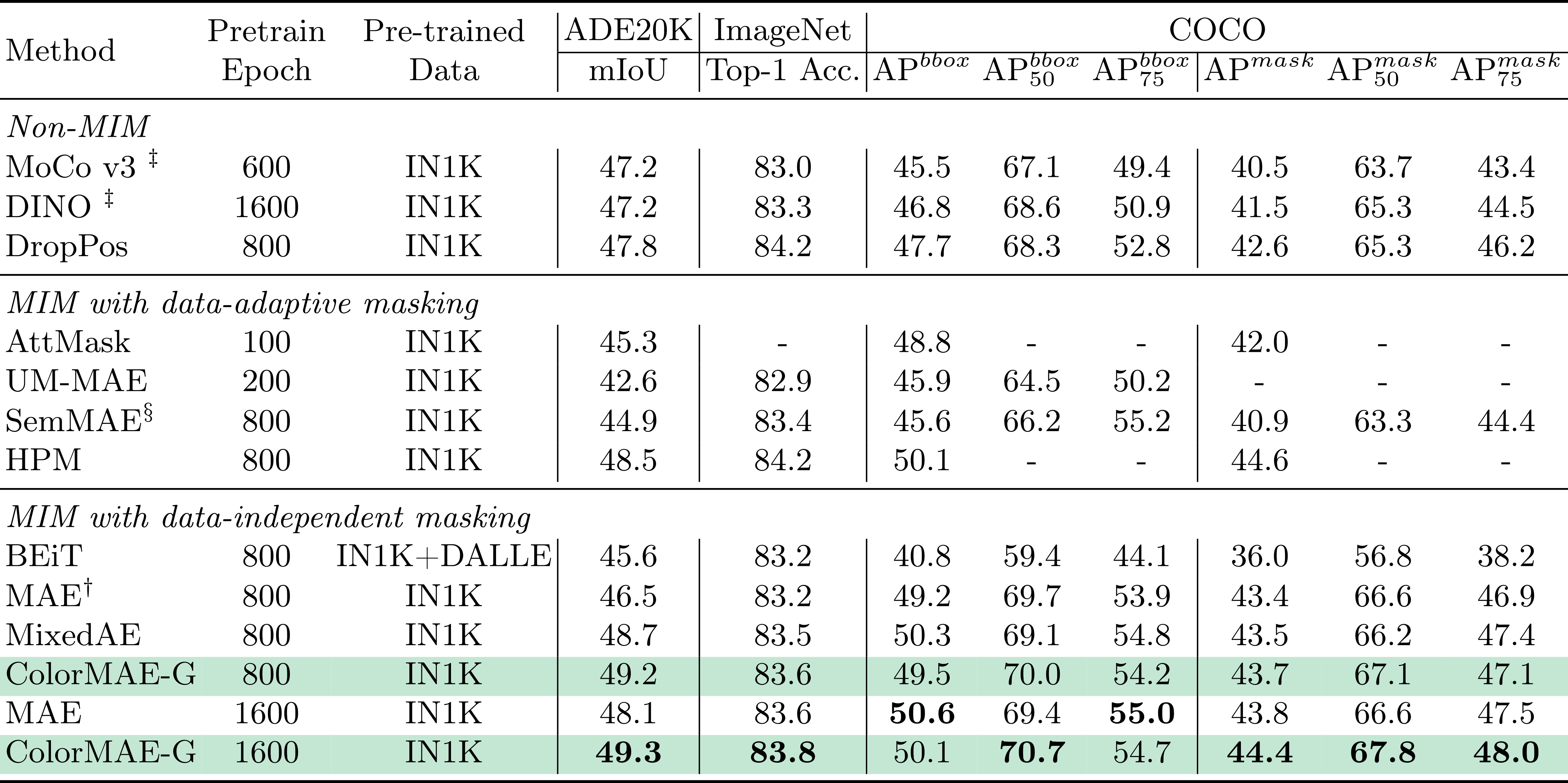
We evaluate the performance of MAE on the downstream tasks mentioned in the previous section when we pre-train with our proposed four types of ColorMAE masks.


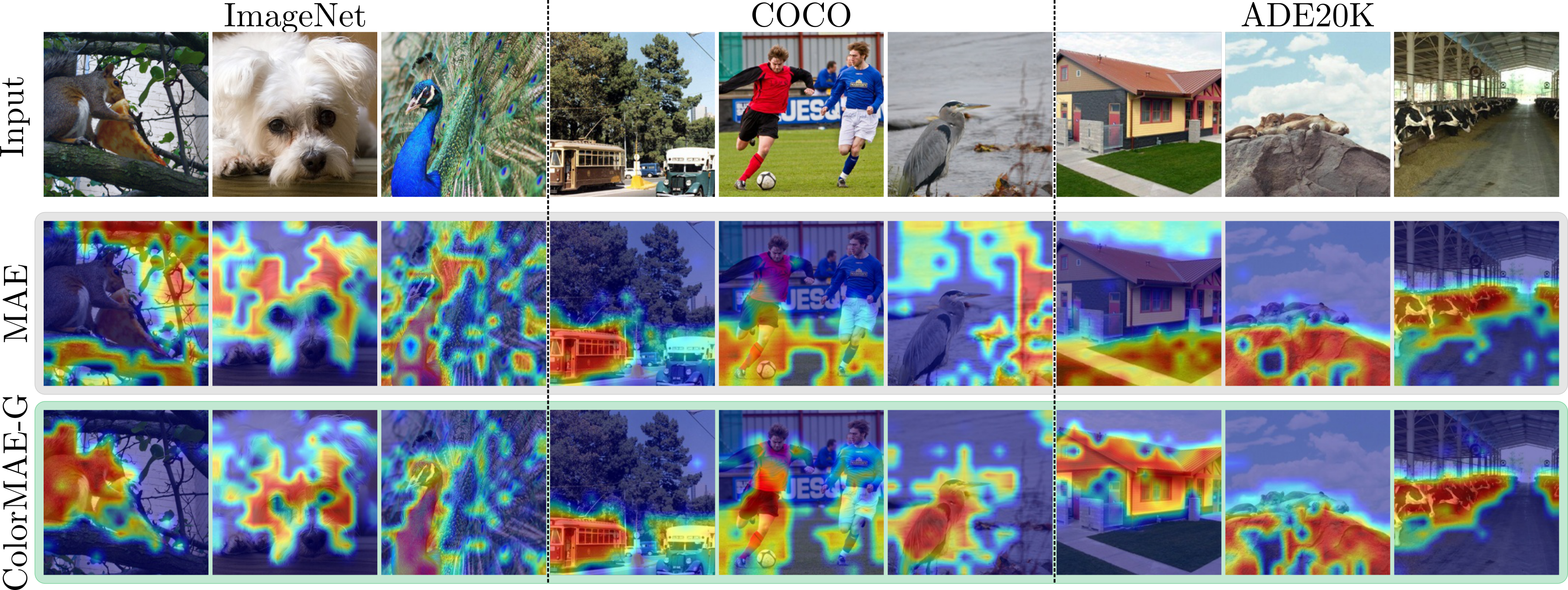
In the Figure below, we show examples of self-attention maps of the [CLS] tokens averaged across the heads of the last layer, for the three different datasets. Here, we show the results for MAE pre-trained using random and our proposed Green masking approach.
![Self-attention of the [CLS] tokens.](/files/ECCV2024ColorMAE/vis_attention.png)

For more results, analysis, visualizations and details, please refer to our paper and supplementary materials.
@article{hinojosa2024colormae,
  title={ColorMAE: Exploring data-independent masking strategies in Masked AutoEncoders},
  author={Hinojosa, Carlos and Liu, Shuming and Ghanem, Bernard},
  journal={arXiv preprint arXiv:2407.13036},
  url={https://arxiv.org/pdf/2407.13036}
  year={2024}
}