ECCV 2026 · Malmö, Sweden Oral · Spotlight

Structured-Noise Masked Modeling for
Video, Audio and Beyond

Aritra Bhowmik1∗Carlos Hinojosa2∗Fida Mohammad Thoker2∗
Bernard Ghanem2Cees G. M. Snoek1

1University of Amsterdam2King Abdullah University of Science and Technology (KAUST)

∗ Equal contribution.

Abstract

Masked modeling has emerged as a robust self-supervised learning framework. However, most methods rely on random masking, which disregards the structural properties of different data modalities. To align with the spatiotemporal and spectral characteristics of video and audio data, we introduce a structured noise-based masking approach. By filtering white noise into different color noise distributions, we generate structured masks that capture modality-specific patterns without requiring handcrafted heuristics or access to the data. Our approach enhances masked video and audio modeling frameworks without any additional computational cost. Experiments show that structured noise masking consistently outperforms random masking, underscoring the value of modality-aware masking strategies for representation learning.

Contributions

Video

3D Green masking (Green3D)

A color-noise masking strategy that produces spatiotemporally coherent masks: visible patches stay clustered in space, while the pattern evolves smoothly across frames.

Audio

Regularized Blue Noise (R-BN)

A 2D blue-noise optimization that enforces a controlled, well-separated distribution of visible spectrogram patches across time and frequency.

Multimodal

Evaluation across modalities

Green3D for the video stream, R-BN for the audio stream. We evaluate on video, audio, and audio-visual benchmarks in both unimodal and multimodal settings.

Method

From white noise to structured noise masks

An input $X$ (image, video, or audio spectrogram) is split into patches and embedded as $X_p = \phi(X) \in \mathbb{R}^{N\times d}$. A masking function $\eta$ turns a noise tensor and a mask ratio $\gamma$ into a binary mask $M \in \{0,1\}^N$, and the encoder only sees the visible tokens. The only thing we change is the noise that goes into $\eta$.

Color noise, in one equation each

Given white noise $n_w \sim \mathcal{N}(0,1)$ and a $d$-dimensional Gaussian kernel $G_\sigma$, three filters give three different families of masks:

Red (low-pass)
$n_r = G_\sigma * n_w$

Smooth, large-scale masked regions.

Blue (high-pass)
$n_b = n_w - G_\sigma * n_w$

Fine-grained, evenly scattered patches.

Green (band-pass)
$n_g = G_{\sigma_1} * n_w - G_{\sigma_2} * n_w$

Mid-sized, spatially clustered masks.

with $\sigma_1 < \sigma_2$. These give the structured masks $M_r = \eta(X_p, n_r, \gamma)$, $M_b = \eta(X_p, n_b, \gamma)$ and $M_g = \eta(X_p, n_g, \gamma)$. Red noise keeps low frequencies and yields smooth, large-scale masked regions; blue noise keeps high frequencies and scatters visible patches finely; green noise balances both and produces mid-sized, clustered masks.
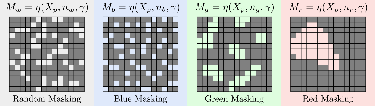
Masks generated from 2D random, blue, green, and red noise.
Masks generated from 2D random, blue, green, and red noise. Gray patches are masked; colored patches are visible.

Green3D noise for video masking

Video masking has to respect both spatial coherence and temporal continuity. VideoMAE and SIGMA use random tube masking, which keeps a static mask across all frames: temporally consistent, but unrelated to the motion in the clip.

We instead apply the green-noise band-pass in 3D, using a white noise tensor $n_w$ and two 3D Gaussian kernels

$$ G_\sigma(\mathbf{x}) = \frac{1}{(2\pi)^{\frac{3}{2}}\sigma^3}\exp\left(-\frac{|\mathbf{x}|^2}{2\sigma^2}\right), \qquad \mathbf{x}=(x,y,z)\in\mathbb{R}^3 . $$

Instead of fixing $(\sigma_1,\sigma_2)$, which produces masks with limited diversity and either overly static or noisy temporal behavior, we randomly sample $(\sigma_1,\sigma_2)$ within $[0.5, 2]$ for each sequence. This generates an ensemble of 3D green noise tensors that remain in the mid-frequency range. Empirically, this stochasticity yields smoother mask evolution and avoids overfitting to a single frequency.
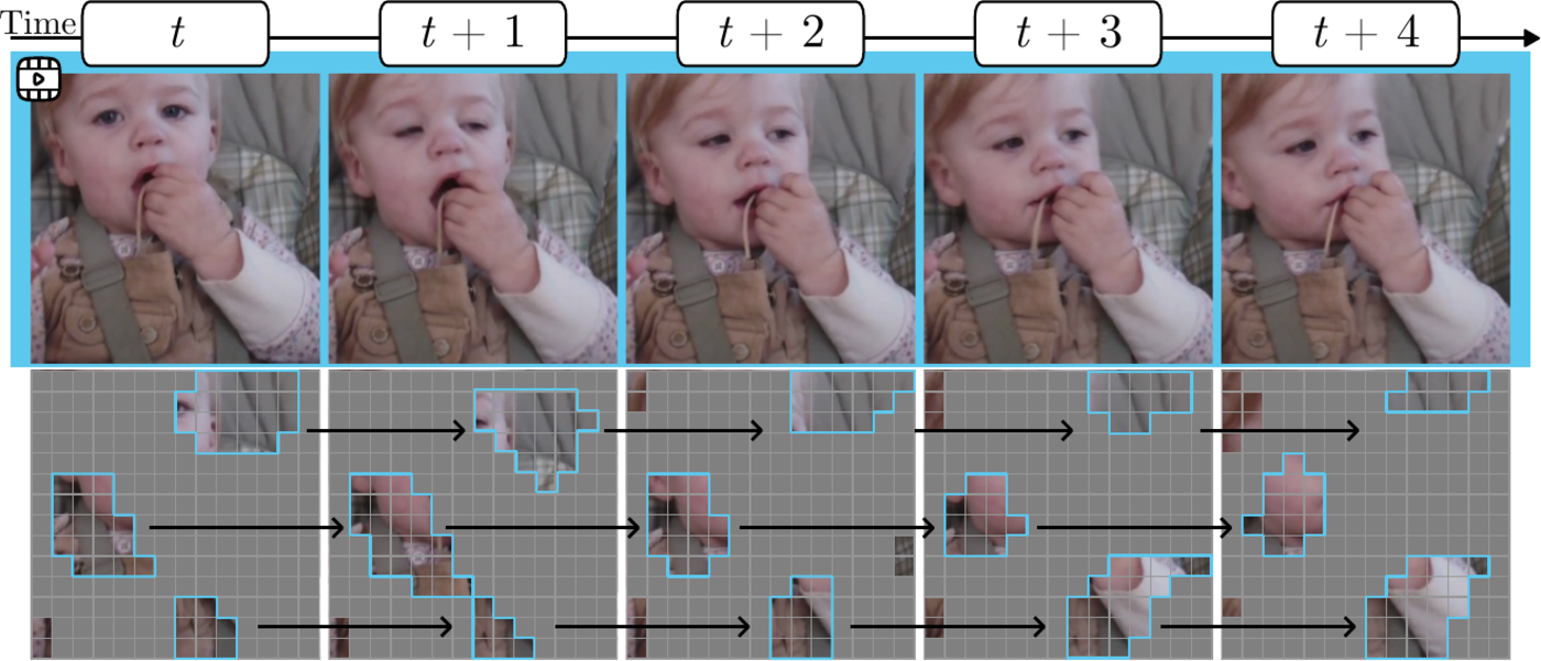
Green3D masks evolving smoothly across consecutive video frames.
How a Green3D mask evolves. Rather than freezing one pattern for the clip, the visible regions shift gradually from frame to frame, following the motion in the scene. This avoids abrupt frame-to-frame changes in what the encoder can see.

Green3D masks are precomputed offline as tensors (e.g. $N\times64\times64\times64$). During training they only undergo flips, normalization and resizing to the token volume (e.g. $14\times14\times8$). These are spatial-domain transforms, so the frequency properties are preserved and masking adds no computational cost at train time.


Regularized Blue Noise (R-BN) for audio masking

Audio spectrograms have a different structure. They encode time–frequency events, and clusters of visible patches, which help in vision, do not correspond to meaningful events here. Blue noise is a better fit because it spreads visible patches more evenly. However, simply high-pass filtering white noise does not explicitly control the separation between visible patches, so small clusters remain.

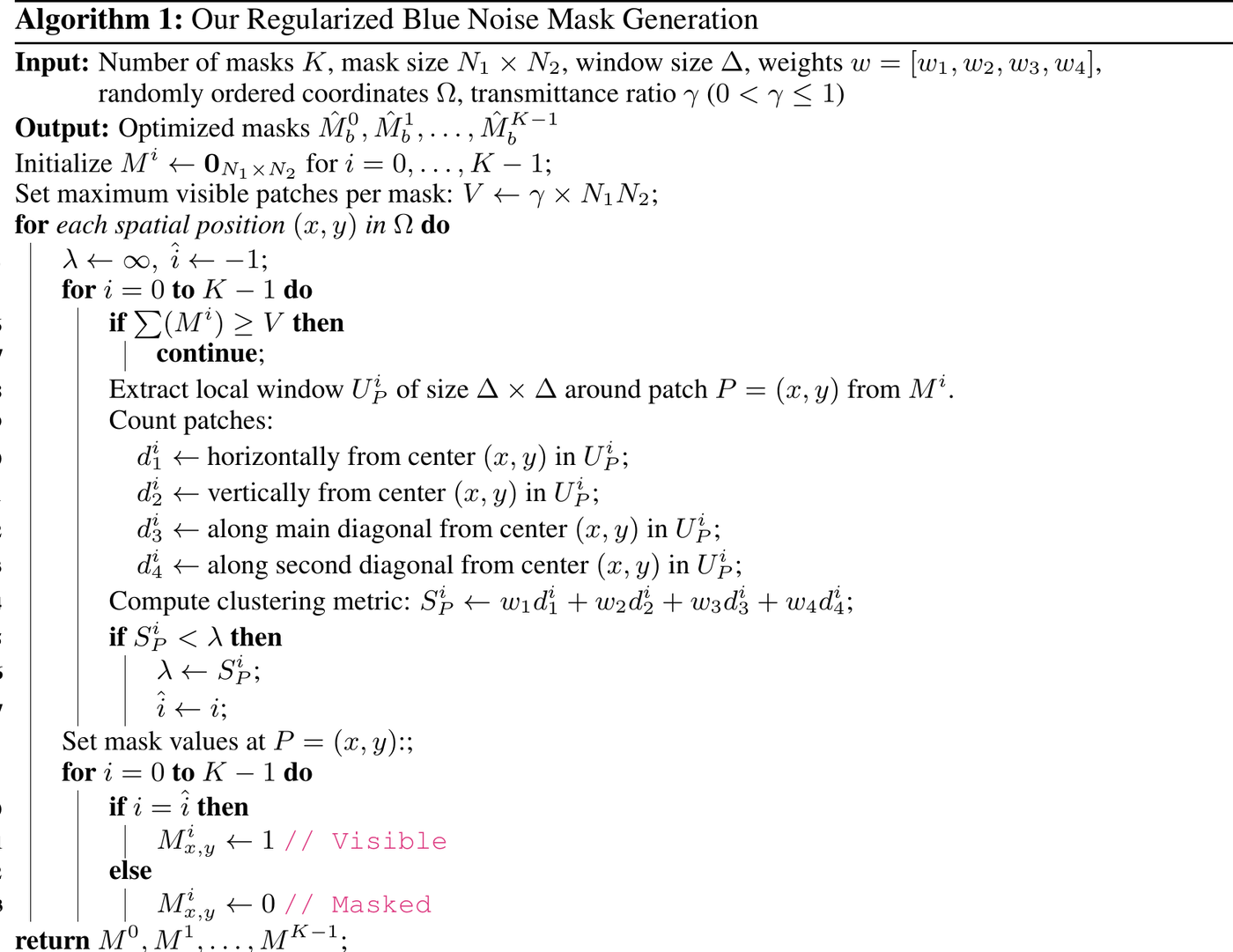
R-BN addresses this with a lightweight optimization. We draw $K$ candidate masks $\{M^i\}_{i=1}^{K}$ by thresholding noise at the target ratio $\gamma$. Then, for each spatial position $P=(x,y)$ in randomized order, we consider a local window $U_P^i \in \mathbb{R}^{\Delta\times\Delta}$ and count visible patches aligned with $P$ along four orientations: horizontal ($d_1^i$), vertical ($d_2^i$) and the two diagonals ($d_3^i, d_4^i$). This gives a clustering score

$$ S_P^i = w_1 d_1^i + w_2 d_2^i + w_3 d_3^i + w_4 d_4^i . $$

The least clustered candidate $\hat{\imath} = \arg\min_i S_P^i$ claims the patch as visible; every other candidate masks it. The loop runs until each mask holds $(1-\gamma)N$ visible patches.

Regularized blue noise masking: clustering metric, initial mask, and optimized mask.
(a) The metric used to measure the concentration of visible patches in a window $U_P^i$. (b) An initial mask $M^i$, with clusters of visible patches. (c) The final mask $\hat{M}_b^i$ from our R-BN algorithm, with more uniformly distributed visible patches and less local clustering.
Pseudocode: Regularized Blue Noise mask generation Algorithm 1: Regularized Blue Noise mask generation pseudocode.
Results

Video, audio, and audio-visual benchmarks

+1.2%VideoMAE on SSv2
top-1 accuracy
+8.7%VideoMAE on DAVIS
segmentation mIoU
+3.1%SIGMA on SEVERE
mean score
+1.1%MaskSpec on AS-20k
audio classification
0additional compute
masks are precomputed

Video: action recognition

We replace the random tube masking in VideoMAE and SIGMA with Green3D, leaving the architecture and every pretraining hyperparameter unchanged. ViT-B backbone, 800 epochs.

Method Masking type SSv2 pretraining K400 pretraining
Data-independent Data-adaptive SSv2 top-1 SSv2 top-1 K400 top-1
VideoMAERandom69.668.580.0
VideoMAE + OursGreen3D70.8+1.269.7+1.280.5+0.5
CMAE-VRandom69.780.2
OmniMAERandom69.569.080.8
MMERandom70.070.581.5
MGMMotion70.671.180.8
MGMAEMotion71.068.981.2
SIGMARandom71.271.181.5
SIGMA + OursGreen3D72.0+0.871.8+0.782.1+0.6

VideoMAE+Green3D matches or surpasses the motion-guided approaches MGM and MGMAE, which require access to motion priors such as optical flow or motion vectors and add computational overhead (MGMAE is about 1.5× slower than VideoMAE). Green3D is data-independent and adds no cost, since the masks are precomputed.

Video: unsupervised video object segmentation

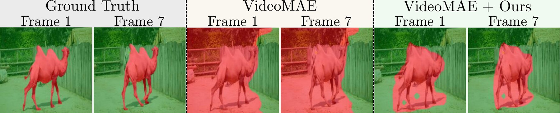
Action recognition pools space–time features into one global clip vector. Segmentation does not: it evaluates whether the encoder produces temporally consistent, object-centric dense features. This is where we observe the largest gains.

Method Clustering Overclustering
YTVOSDAVISYTVOSDAVIS
VideoMAE34.129.561.356.2
VideoMAE + Ours35.6+1.538.2+8.762.5+1.558.2+2.0
MGM36.636.561.256.6
MGMAE34.531.060.157.5
SIGMA41.133.167.159.0
SIGMA + Ours42.1+1.334.2+1.268.4+1.360.0+1.0

mIoU under the protocol of Time Does Tell; ViT-B pretrained on K400, official checkpoints for all prior work.

Unsupervised video object segmentation on DAVIS: ground truth, VideoMAE, and VideoMAE + Green3D.
Qualitative results on DAVIS. Green3D masking produces sharper, more object-centric segmentations and is more temporally consistent across frames than the VideoMAE baseline.

Video: SEVERE generalization benchmark

Eight experiments across four axes of generalization: domain shift, sample efficiency, action granularity, and task shift. All methods pretrained on K400 with a ViT-B backbone.

Method Domain shift Sample efficiency Action granularity Task shift Mean
SSv2Gym99 UCF(103)Gym(103) FX-S1UB-S1 UCF-RC↓Charades
VideoMAE68.686.674.625.936.674.30.17217.258.3
VideoMAE + Ours69.788.175.029.938.674.80.17018.259.6+1.3
MVD70.082.567.117.531.350.50.18416.152.1
MGMAE68.987.277.224.133.779.50.18117.958.8
MGM71.189.178.426.438.686.90.15222.562.2
MME70.189.779.229.855.587.20.15523.665.0
SIGMA70.989.784.128.055.179.90.16923.164.2
SIGMA + Ours71.890.785.035.056.585.90.16327.567.3+3.1

For UCF-RC, lower is better: the metric reports mean repetition-counting error.

Averaged over the eight settings, Green3D raises the SEVERE mean score by 1.3 points for VideoMAE and by 3.1 points for SIGMA, with improvements on all four axes of generalization.

Audio

R-BN replaces the default random masking inside AudioMAE and MaskSpec, leaving the rest of each framework unchanged. ViT-B, 80% masking during pretraining on AudioSet-2M, 30% during fine-tuning.

MethodAS-20kAS-2MESC-50SPC-2
SS-AST31.088.898.0
MaskSpec32.347.189.697.7
MaskSpec + Ours33.4+1.147.6+0.590.4+0.898.2+0.5
MAE-AST30.690.097.9
Audio-MAE*36.146.394.198.3
Audio-MAE + Ours36.8+0.747.2+0.994.6+0.598.7+0.4

* Results from our own evaluation. The public AudioSet test split has changed over time due to YouTube removals, so we re-evaluate every baseline on the same current split for a fair comparison.

R-BN improves both frameworks on all four benchmarks. Unlike MaskSpec, which relies on predefined time–frequency rules, or MAE-AST, which uses additional speech data, R-BN needs no supervision or access to the data.

Audio-visual

Inside CAV-MAE, we use Green3D for the video stream and R-BN for the audio stream. 75% masking on both modalities, ViT-B, 25 epochs of pretraining on VGGSound.

MethodAudioVideoAudio-Video
MBT52.351.264.1
CAV-MAE*58.545.664.3
CAV-MAE + Ours59.1+0.646.4+0.864.9+0.6

* Results from our own evaluation, following the authors' publicly released VGGSound pipeline.

Since CAV-MAE uses random masking for both streams, structured noise can be used as a drop-in replacement without adding objectives or computational cost. We observe gains in the unimodal settings as well as in the joint audio-visual setting.

Ablations

Which color, and why 3D?

All ablations use smaller subsets: mini-Kinetics (25% of K400) and mini-SSv2 (50% of SSv2) for video, AS-20k and ESC-50 for audio.

The best mask color differs between video and audio

3D masks for video

Color mask$\mathcal{L}_{\text{recon}}$mini-Kineticsmini-SSv2
Random0.6751.652.8
Blue0.4150.952.1
Red0.8551.052.3
Green0.6052.754.5

2D masks for audio

Color mask$\mathcal{L}_{\text{recon}}$AS-20kESC-50
Random0.5236.194.1
Blue0.4536.594.2
Red0.6135.592.6
Green0.5736.494.1

For video, green gives the best balance between reconstruction difficulty and solvability in our experiments (loss 0.60). Blue lowers the reconstruction loss the most (0.41), which appears to make the task too easy, while red raises it (0.85); both give lower accuracy than green. For audio, the ordering changes: blue performs best, green gives no benefit over random, and red degrades accuracy. The ranking of colors is therefore not the same across the two modalities.

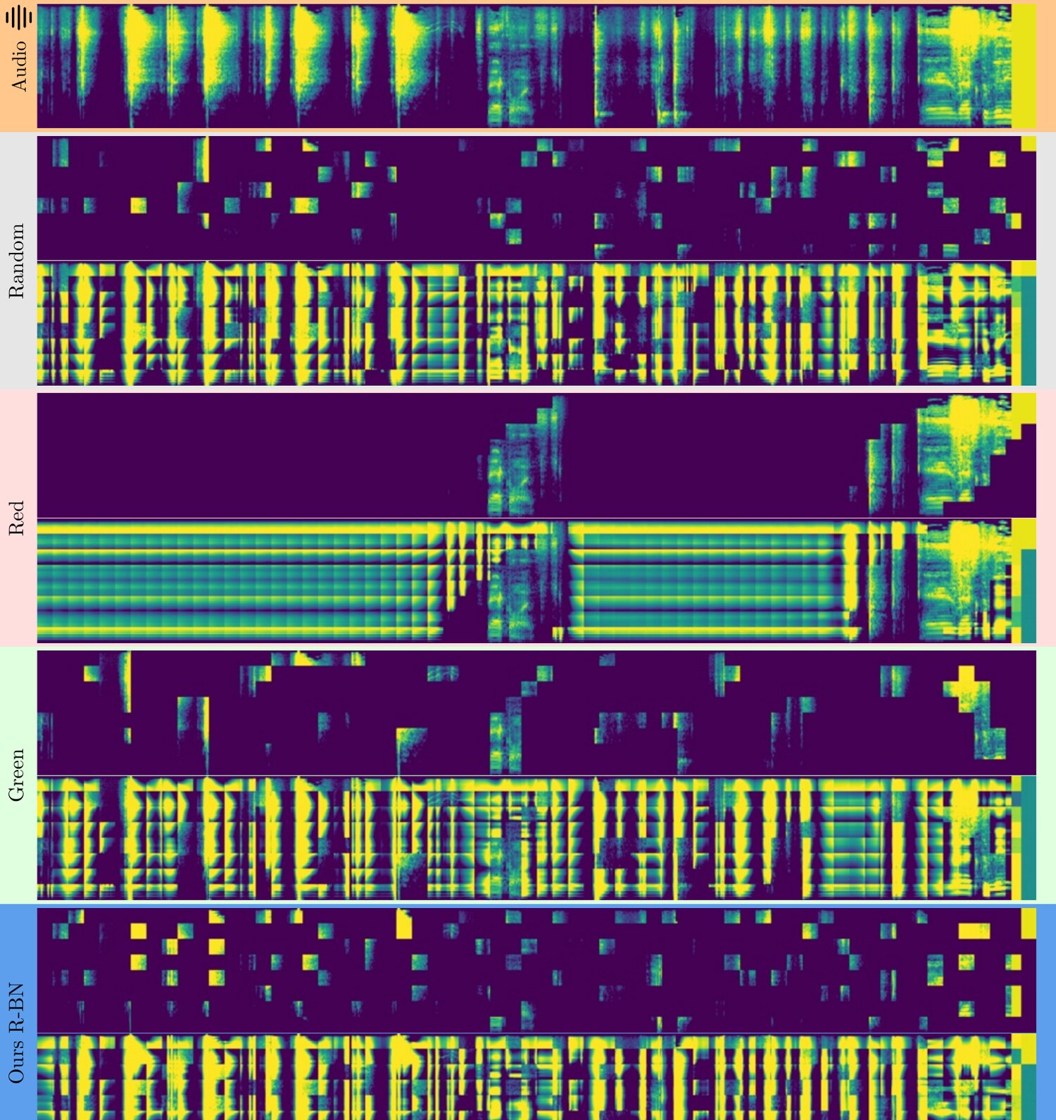
Spectrogram reconstruction under random, red, green, and R-BN masking.
Spectrogram reconstruction under different masking strategies (AudioMAE, masking ratio 0.8). Random masking leads to scattered reconstructions, while red and green noise introduce artifacts that distort the frequency structure. Regularized Blue noise masking produces a more balanced reconstruction, closer to the spectral distribution of the input.

Blue vs. R-BN, and 3D vs. 2D

Audio: regularizing blue noise

Masking type$\mathcal{L}_{\text{recon}}$AS-20kESC-50
Blue0.4536.594.2
R-BN0.4936.894.6

Video: 3D vs. 2D structure

Masking type$\mathcal{L}_{\text{recon}}$mini-Kineticsmini-SSv2
Tube0.6751.652.8
Green2D0.7351.952.9
Green3D0.6052.754.5

Applying the same 2D green mask to every frame gives only a small improvement over random tube masking (+0.3 / +0.1). Independently sampling a fresh 2D green mask per frame does not help either (51.7 / 53.1). In our experiments the gain comes from coherent 3D spatiotemporal structure, which suggests that extending structured noise masking from images to video is not a trivial adaptation.

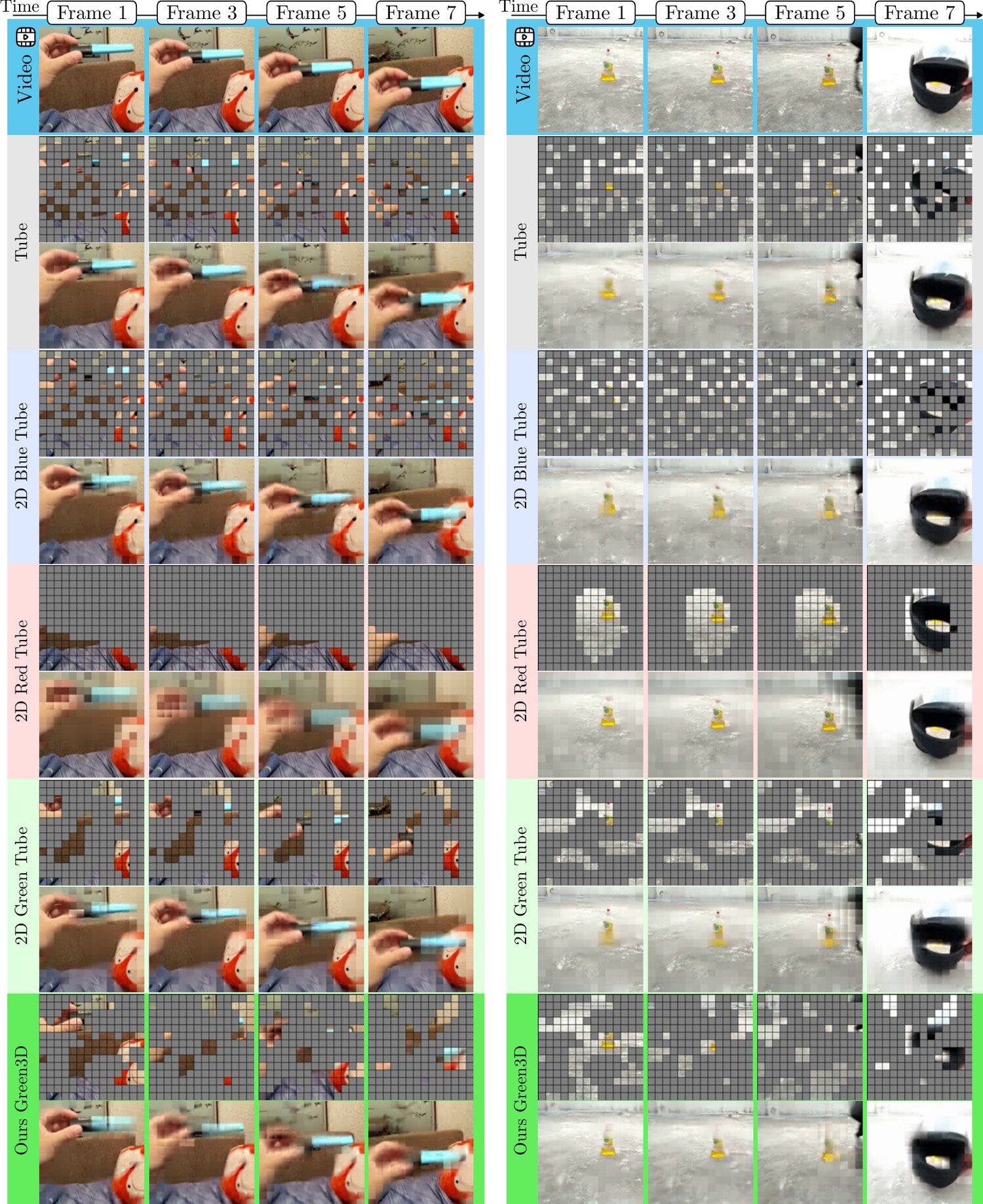
Video reconstruction under tube, 2D blue, 2D red, 2D green, and Green3D masking.
Video reconstruction under different masking strategies (VideoMAE pretrained on SSv2, masking ratio 0.75). Tube masking does not align with the structures in the video; 2D noise-based masking adds spatial coherence but lacks temporal consistency. Green3D follows the spatiotemporal structure, preserving motion continuity across frames.

Fine-grained tasks across 3D mask colors

Method SEVERE Clustering Overclustering
Gym99FX-S1UB-S1Charades YTVOSDAVISYTVOSDAVIS
Random72.035.771.314.229.725.356.243.9
Red3D72.537.573.015.431.225.954.748.6
Blue3D73.434.769.315.831.325.555.644.1
Green3D75.438.572.616.032.927.360.050.9

Red3D and Blue3D improve some individual metrics, while Green3D is the strongest overall across these tasks.

Masking ratio. VideoMAE typically peaks near 90% masking and AudioMAE near 80%. Green3D and R-BN follow the same trends: gains grow from 80% to 90% for video, and performance peaks near 80% for audio. The masking ratios used with random masking therefore carry over.

Taken together, these ablations point in the same direction: the choice of structured noise matters, and the choice that works best is not the same for video and audio.

Cite this work

Structured-Noise Masked Modeling (ECCV 2026)

@inproceedings{bhowmik2026structured,
  title     = {Structured-Noise Masked Modeling for Video, Audio and Beyond},
  author    = {Bhowmik, Aritra and Hinojosa, Carlos and Thoker, Fida Mohammad
               and Ghanem, Bernard and Snoek, Cees G. M.},
  booktitle = {European Conference on Computer Vision (ECCV)},
  year      = {2026}
}

This work builds directly on ColorMAE (ECCV 2024), which introduced color noise-based masking for static images. If you use our masking strategies, please consider citing it as well.

ColorMAE (ECCV 2024)

@InProceedings{Hinojosa_2024_ECCV,
    author    = {Hinojosa, Carlos and Liu, Shuming and Ghanem, Bernard},
    title     = {ColorMAE: Exploring data-independent masking strategies in Masked AutoEncoders},
    booktitle = {European Conference on Computer Vision (ECCV)},
    month     = {September},
    year      = {2024},
    doi       = {10.1007/978-3-031-72661-3_25}
}

Acknowledgements

This work has been financially supported by TomTom, the University of Amsterdam, and the allowance of Top consortia for Knowledge and Innovation (TKIs) from the Netherlands Ministry of Economic Affairs and Climate Policy. Cees G. M. Snoek is also (partially) funded by the Horizon Europe project ELLIOT (GA No. 101214398). The research was also supported by funding from King Abdullah University of Science and Technology (KAUST) Center of Excellence for Generative AI, under award number 5940. For computing time, this research used Ibex, managed by the Supercomputing Core Laboratory at KAUST in Thuwal, Saudi Arabia. We also extend our gratitude to the anonymous reviewers for their valuable feedback and insightful suggestions during the rebuttal stage, which considerably improved this work.